Annual directional plots can be used for analysing ambient air-pollution measurements near power stations

These bi-polar plots show monitored hourly SO₂ concentrations in the Aire Valley in Yorkshire. See below for more details.

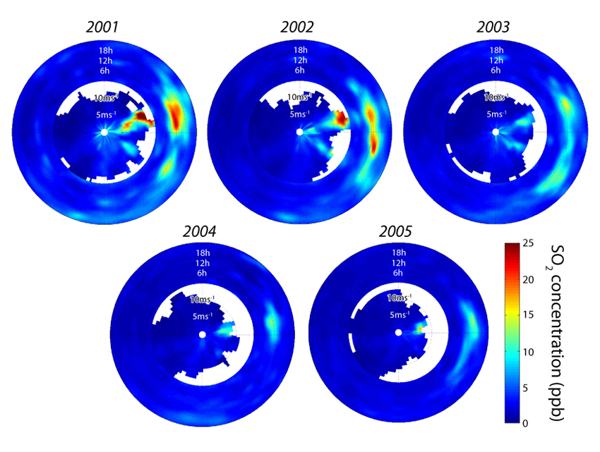
The plots show the direction of sources delivering raised impacts, but they also show other interesting features of the data: Each plot contains an 'inner' bi-polar plot and an 'outer' bi-polar plot. The radial axis of the inner plot measures wind speed and ranges from 0 to 15m/s. This descibes how ambient concentrations of SO₂ vary with wind speed, and shows that raised concentrations tend to occur when there are higher wind speeds from the directions of the power stations.

The radial axis of the outer plot measures time-of-day and ranges from 0 to 2300 hours. This describes how ambient concentrations of SO₂ vary diurnally, and shows that raised concentrations from the directions of the power stations tend to occur around the middle of the day and during the early afternoon. These raised concentration features comprise a dispersion 'signature', which is typical of plumes from elevated stacks.

Changes in the magnitude of concentration 'hot-spots' between years represent changes in the emission performance of polluting sources

See our Case Studies to find out how these techniques have been applied to real-life sources, data and management decisions.

Bi-polar plots can also be used to identify clear and frequent source signals, so that air-quality monitoring data can be analysed in more detail

More detailed analyses would permit additional information to be extracted from ambient data and used for air-quality management purposes

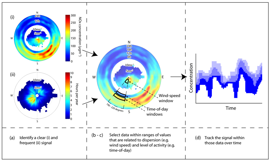
The above figure shows a multi-stage process for selecting ambient air-quality data 'conditionally', i.e. selecting hourly concentrations based on the corresponding meteorology and level of source activity. These 'conditionally-selected' data can then be analysed over time for evidence on the emission performance of air pollution sources

The schematic shows how NO₂ monitoring data near a motorway can be visualised in order to identify ranges of data that contain clear and frequent source signals (stage a). These data can be selected from within meteorological, and activity-level 'windows'. For example, Stage b shows how windows have been defined around particular ranges of wind direction, wind speed and time-of-day. These data are then analysed over time and examined for evidence of source performance or policy outcomes

The data can be selected for consistent dispersion conditions, in order to eliminate or reduce the effect of variations in meteorology. Selecting the data for consistent times of the day/week helps to reduce the effect of variations in activity-level

See our Case Studies to find out how these techniques have been applied to real-life sources, data and management decisions.

The 'Dispersion Calendar' has been developed as a means of dissecting and comparing meteorology and ambient air-quality data. These data may be based on measurements or model predictions

The dissection scheme of the Calendar is based on specific combinations of hourly meteors that are related to dispersion - time-of-day, season, wind speed and cloud cover

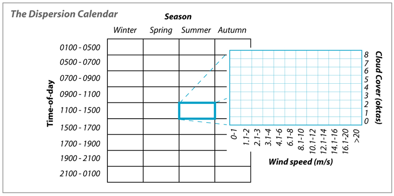
The calendar can be used to learn more about the sources of raised pollution impacts. In particular, it can be used to identify timings and dispersion conditions of raised-impact situations

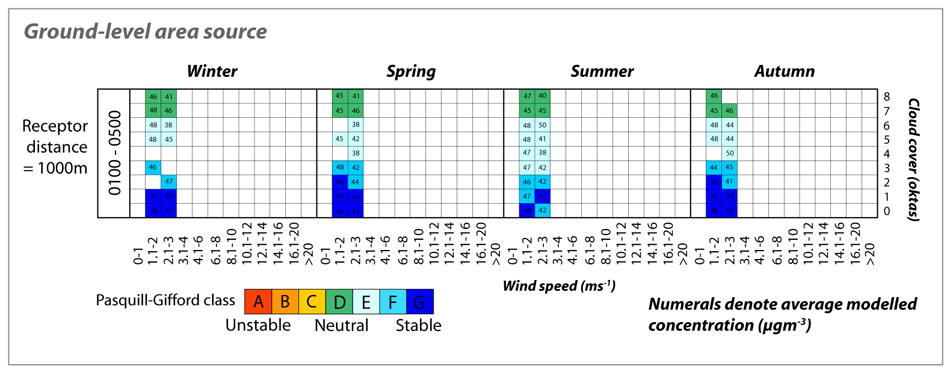
The examples below show the timing and dispersion conditions of the highest 10% of modelled concentrations from 2 sources: a tall 200m stack and a ground-level area source

For example, raised ground-level concentrations from a tall stack tend to occur under high-wind-speed neutral 'knock-down' conditions, and also under more convective unstable 'plume-looping' conditions around the middle of the day

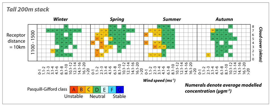
By contrast, ground-level concentrations from a low-level area source tend to be raised during low-wind-speed stable conditions

Where the causes of raised pollution impacts are unclear, the Calendar can therefore be used to diagnose the nature of raised-impact situations, in order to help with source attribution

See our Case Studies to find out how these techniques have been applied to real-life sources, data and management decisions.

Conventional methods of comparing modelled and monitored data in order to assess model performance do not provide a detailed account of model performance.

This is because they tend to compare bulk statistics that do not describe model performance for particular dispersion conditions or stages of activity cycles.

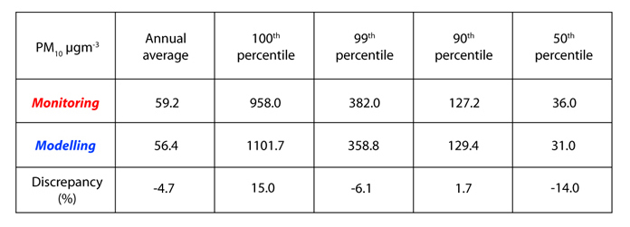
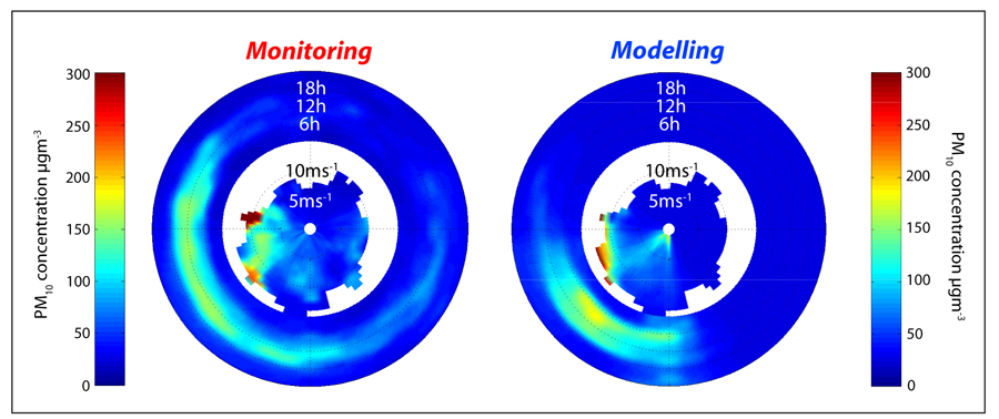
An additional and more refined 'conditional' validation is shown here that checks if the temporal and directional features of ambient data are re-produced by the model.

The bi-polar plots compare monitored and modelled concentrations of PM₁₀ near a mixed industrial site. The comparisons show that there is reasonable agreement between the magnitudes, temporal variations, and directional dependencies of ambient PM₁₀ concentrations.

See our Case Studies to find out how these techniques have been applied to real-life sources, data and management decisions.

Coming soon